Acknowledgements
We thank Gao Jun Wu, a PhD Candidate of the Stanford FPAL Lab for his expert technical advisory on the project as a whole, and in helping us to organize and plan the research direction. We also thank Professor Seongkyu Lee, director of the UC Davis CFPA Lab, for his advisory regarding computational methods and validation. Additionally, we would like to thank Dr. Nikolas Zawodny of NASA's Langley Research Center for his suggestion to base our propeller designs around those discussed in this paper. That is our current objective regarding computational validation.
Overview
Unmanned aerial vehicles (UAVs) are becoming more commonly used in populated areas, raising concerns about noise pollution generated from their propellers. We seek to investigate the acoustic performance of unconventional propeller designs—specifically toroidal and uneven-blade spaced propellers—for their potential in reducing psychoacoustic annoyance.
Initial Results
Our experimental results show that our designs noticeably reduced psychoacoustic annoyance while showing small improvements in thrust. We hope to extend our results by accessing an anechoic chamber to conduct acoustics testing and developing a standardized methodology for our propeller designs.
Current TUBAA Propellers
.png)
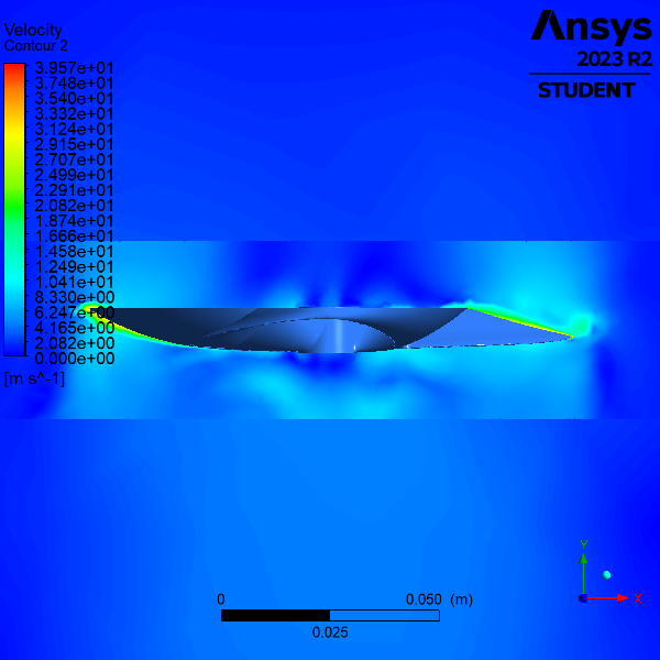
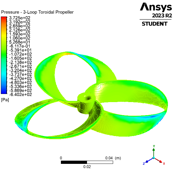
Our findings indicate a clear correlation between unconventional propeller design parameters and their aeroacoustic performance. Uneven blade spacing and toroidal geometries have shown potential in reducing propeller noise without significantly compromising thrust or efficiency. The results from our CFD simulations were in agreement with our experimental data, showing a clear reduction in vorticity for the toroidal propellers, as compared to conventional.
Propeller Curve Design
We are completely overhauling our design methodology for the experimental propellers, to be based around different parameters and controls. In these initial designs, which we FDM printed and tested for thrust, stiffness, and acoustics, our method involved using a sequence of airfoil profiles (consistent among all tested propellers) and sweeping them along rails.
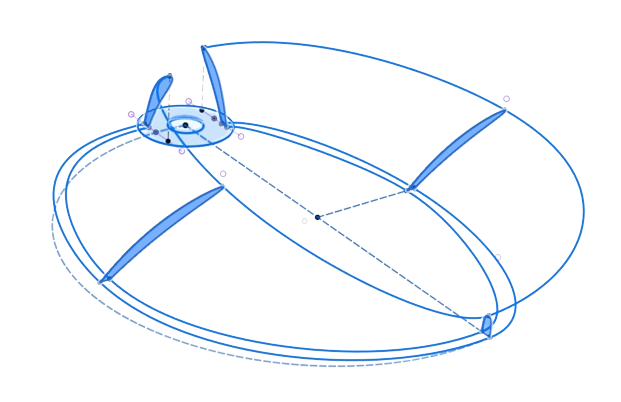
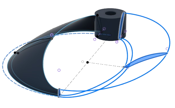
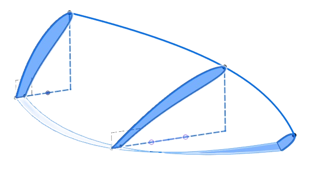
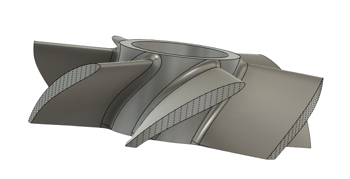
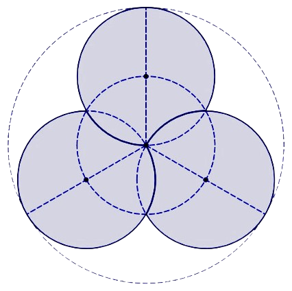
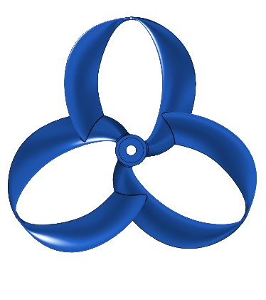
For the conventional propellers, these rails were simply six radii, equally spaced from each other. For the toroidal propeller, these rails composed of three arcs, constructed geometrically with one outer circle of radius r and four circles of radius r/2, as shown below.

Acoustic Analysis
Understanding and analyzing propeller noise is crucial. This section explains the key concepts and methods we used in our initial, experimental acoustic analysis.
Fast Fourier Transform (FFT)
The FFT is a computational algorithm used to convert a signal from its original domain (often time or space) into a representation in the frequency domain. Mathematically, the FFT can be expressed as:
\[ X(k) = \sum_{n=0}^{N-1} x(n) \cdot e^{-\frac{2\pi i}{N} kn} \]
where \( x(n) \) is the original signal, \( N \) is the total number of samples, and \( X(k) \) is the resulting frequency domain representation. Here's a Python implementation of the FFT using the NumPy library:
time_signal = np.array([...])
frequency_signal = np.fft.fft(time_signal)
frequencies = np.fft.fftfreq(len(time_signal))
In the above code, time_signal is an array representing the signal in the time domain. The fft function transforms this signal into the frequency domain, resulting in the frequency_signal array. The fftfreq function then computes the corresponding frequencies.
Sound Pressure Level (SPL)
The SPL is a logarithmic measure used to quantify sound intensity. It is calculated using the formula:
\[ \text{SPL} = 20 \cdot \log_{10}\left(\frac{p}{p_0}\right) \, \text{dB} \]
where \( p \) is the root mean square sound pressure, and \( p_0 \) is the reference sound pressure, typically \( 20 \mu Pa \) in air. Below is a Python code snippet to calculate the SPL:
p_rms = np.sqrt(np.mean(np.square(pressure_signal)))
SPL = 20 * np.log10(p_rms / p_ref)
Overall Sound Pressure Level (OASPL)
The OASPL provides a single value that represents the total acoustic energy of a sound spectrum, integrating the SPL over all frequencies. It is calculated as:
\[ \text{OASPL} = 10 \cdot \log_{10}\left(\sum_{i} 10^{\frac{SPL_i}{10}}\right) \, \text{dB} \]
The Python code to calculate OASPL is shown below:
OASPL = 10 * np.log10(np.sum(10 ** (SPL / 10)))A-Weighting
We use A-Weighting on acoustic data in order to evaluate the percieved annoyance for human listeners. A-Weighting is a frequency weighting standard used to mimic the human ear's response to different frequencies, with more emphasis on frequencies between 1 to 6 kHz. The A-Weighted SPL can be calculated using specific weighting filters applied to the frequency components of the sound.
Blade Harmonics
Blade harmonics are specific frequencies in the sound spectrum that correspond to the rotational speed of the propeller and its multiples. They are calculated based on the number of blades (\( B \)) and the rotation speed (\( RPM \)):
\[ f_b = \frac{B \cdot RPM}{60} \, \text{Hz} \]
where \( f_b \) is the blade passing frequency. The harmonics are found at integer multiples of this frequency. The Python code to calculate the blade passing frequency is as follows:
blade_passing_frequency = (number_of_blades * RPM) / 60Appendix
